偏振是一种重要的光学现象,振动方向对于传播方向的不对称性叫做偏振,它是横波区别于其他纵波的一个最明显的标志,只有横波才有偏振现象。光波是电磁波,因此,光波的传播方向就是电磁波的传播方向。光波中的电振动矢量E和磁振动矢量H都与传播速度v垂直,因此光波是横波,它具有偏振性。具有偏振性的光则称为偏振光。
虽然可以想象一束光波是由振荡的电场和磁场以恰当的角度一起在空间中移动,但没有可视化的仿真仍然会让人产生困惑。为了描述电场、磁场与光传播方向的关系,我首先进行了如下线偏振光的可视化仿真:
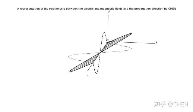
线偏振光可视化结果
通过仿真结果可见,光波电矢量的振动方向只局限在一确定的平面内,这种偏振光被称为平面偏振光,又因振动的方向在传播过程中为一直线,故又称线偏振光。
源代码如下:
import scipy as sc
import matplotlib as mpl

from mpl_toolkits.mplot3d import Axes3D

import matplotlib.pyplot as plt
from matplotlib.patches import FancyArrowPatch
from mpl_toolkits.mplot3d import proj3d

class Arrow3D(FancyArrowPatch):
    def __init__(self, xs, ys, zs, *args , **kwargs):
        FancyArrowPatch.__init__(self, (0,0), (0,0), *args , **kwargs)
        self._verts3d = xs, ys, zs

    def draw(self, renderer):
        xs3d , ys3d , zs3d = self._verts3d
        xs, ys, zs = proj3d.proj_transform(xs3d , ys3d , zs3d , renderer.M)
        self.set_positions((xs[0],ys[0]) ,(xs[1],ys[1]))
        FancyArrowPatch.draw(self, renderer)


fig = plt.figure()
fig.set_size_inches(12,7)
ax = fig.add_subplot(1,1,1,projection='3d')

polAng = sc.pi/4
# Plot the wave in the xy plane
t = sc.linspace(0, 2*sc.pi ,512)
x = sc.sin(t)*sc.cos(polAng)
y = sc.sin(t)*sc.sin(polAng)
xx = sc.zeros(t.size)
yy = sc.zeros(t.size)
#plt.hold(True)
ax.plot(t, x, yy, 'k', ls='dotted') # The x−component
ax.plot(t, xx, y,'k', ls='dashed') # The y−component

# Plot the E vectors
tv = sc.linspace(0,2*sc.pi ,16)
xv = sc.sin(tv)*sc.cos(polAng)
yv = sc.sin(tv)*sc.sin(polAng)

# The E−vector and its envelope
for i in range(len(tv)):
    a = Arrow3D([tv[i], tv[i]], [0, xv[i]], [0, yv[i]], mutation_scale=15, lw=1, arrowstyle="<-", ls='dashed', color ='k')
    ax.add_artist(a)
ax.plot(t, x, y, color='k')

# The x, y and t axes
a = Arrow3D([-0.5,-0.5], [0,1.25], [0,0], mutation_scale=15, lw=1,arrowstyle="<-", color="k")
ax.add_artist(a)
ax.text(-0.5, 1.25,0, r'$hat{x}$')
a = Arrow3D([-0.50,-0.50], [0,0], [0,1.25], mutation_scale=15, lw=1, arrowstyle="<-", color="k")
ax.add_artist(a)
ax.text(-0.5, 0, 1.35, r'$hat{y}$')
a = Arrow3D([-0.5,2.75*sc.pi], [0,0], [0,0], mutation_scale=15, lw=1, arrowstyle="<-", color="k")
ax.add_artist(a)
ax.text(2.85*sc.pi, 0,-0.2,r'$t$')

ax.set_xlim(0,7.5)
ax.set_ylim(-1.2, 1.2)
ax.set_zlim(-1.2, 1.2)
ax.set_xticklabels ([])
ax.set_yticklabels ([])
ax.set_zticklabels ([])
ax.set_title ('A representation of the relationship between the electric and magnectic fields and the propagation direction by CHEN')
plt.axis('off')
ax.elev=25
ax.azim=10
plt.show()
同理,圆偏振光可视化结果如下:
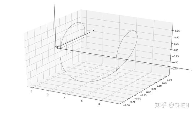
圆偏振光可视化结果
源代码如下:
import scipy as sc
import matplotlib as mpl

from mpl_toolkits.mplot3d import Axes3D

import matplotlib.pyplot as plt
from matplotlib.patches import FancyArrowPatch
from mpl_toolkits.mplot3d import proj3d

class Arrow3D(FancyArrowPatch):
    def __init__(self, xs, ys, zs, *args , **kwargs):
        FancyArrowPatch.__init__(self, (0,0), (0,0), *args , **kwargs)
        self._verts3d = xs, ys, zs

    def draw(self, renderer):
        xs3d , ys3d , zs3d = self._verts3d
        xs, ys, zs = proj3d.proj_transform(xs3d , ys3d , zs3d , renderer.M)
        self.set_positions((xs[0],ys[0]) ,(xs[1],ys[1]))
        FancyArrowPatch.draw(self, renderer)
fig = plt.figure()
fig.set_size_inches(12,7)
ax = fig.add_subplot(1,1,1,projection='3d')

polAng = sc.pi/4


# Plot the wave in the xy plane
t = sc.linspace(0, 3*sc.pi ,512)
x = sc.cos(t)
y = sc.sin(t)
#plt.hold(True)
# Plot the E vectors
tv = sc.linspace(0,2*sc.pi ,16)
xv = sc.cos(tv)
yv = sc.sin(tv)

# The E−vector and its envelope
for i in range(len(tv)):
    a = Arrow3D([tv[i],tv[i]], [0 ,xv[i]], [0,yv[i]], mutation_scale=15, lw=0.35, arrowstyle="<-", color='k')
    ax.add_artist(a)
    ax.plot(t, x, y, color='k', lw=0.5)
    # The x, y and t axes
    a = Arrow3D([-0.5,-0.5], [0,1.5], [0,0], mutation_scale=15, lw=1,arrowstyle="<-", color="k")
    ax.add_artist(a)
    ax.text(-0.5, 1.6,0, r'$hat{x}$')
    a = Arrow3D([-0.50,-0.50], [0,0], [0,1.75], mutation_scale=15, lw=1, arrowstyle="<-", color="k")
    ax.add_artist(a)
    ax.text(-0.5, 0, 1.85, r'$hat{y}$')
    a = Arrow3D([-0.5,5.75*sc.pi], [0,0], [0,0], mutation_scale=15, lw=1, arrowstyle="<-", color="k")
    ax.add_artist(a)
    ax.text(5.85*sc.pi, 0,-0.2,r'$t$')
    plt.show()
到目前为止,我们还只介绍了关于偏振光的最粗浅认识,如何应用不同偏振态的光源进行深层次的光学探索还未涉及。
比如,如何利用不同偏振态的光束相互干涉实现超精密位移测量?自然光和偏振光的区别还有什么?和偏振相关的光学器件,如起偏器、检偏器功用的器件,其在光路中如何用数学公式进行表示?如何用琼斯矩阵推导出一条完整的光路方程?

总之,更多的细节还需读者根据自己的科研需要自行探索,本期文章仅做抛砖引玉之用。